In Zhang et al. (2022), we introduce a method allowing to compute synthetic (or average) signals issued from multiple correlated and/or even non-stationary signals. In a nutshell, this method minimizes a weighted average of the wavelet variance of the synthetic signal whose weights can be chosen depending on the application at hand. This method is illustrated with gyroscopes which often contain non-stationary processes such as random walks. This package implements the method of Zhang et al. (2022), called Scale-wise Variance Optimization or SVO, as well as the approach of Vaccaro and Zaki (2017), which is used as a comparison.
Real Gyroscope Data Analysis
We consider the real gyroscope data considered in Zhang et al. (2022), where a virtual gyroscope is created by fusing 12 real MEMS from two device families, InvenSense ICM-20689 and Bosch BMI055. The employed data is included in the package and can be loaded as follows:
We first need to choose which scales we would like to minimize in the wavelet variance plot. In the SVO proposed in Zhang et al. (2022), this is obtained by choosing non-negative weights on the scales that sum to one. For example, if one is interested in minimizing the large scales of the wavelet variance, suitable weights can be obtained as follows:
n_scales = log2( nrow(Xt) ) - 1
tau = 1:n_scales

weights = exp(tau-15)/(1 + exp(tau-15))
weights = weights/sum(weights)

plot(NA, xlim = range(tau), ylim = range(weights), xlab = "Wavelet variance scales", ylab = "Weight", xaxt="n")
p10s = seq(0,log10(2^(tail(tau,1))))

abline(v = log2(10^p10s), col = "grey", lt = 2 )
abline(h = seq(0,0.15,0.05), col = "grey", lt = 2 )
lines(tau, weights, lwd = 1.3)

# plot x axis labels in samples (powers of 10)
axis(1, at = log2(10^p10s), labels = sapply(p10s, function(i) as.expression(bquote(10^ .(i)))))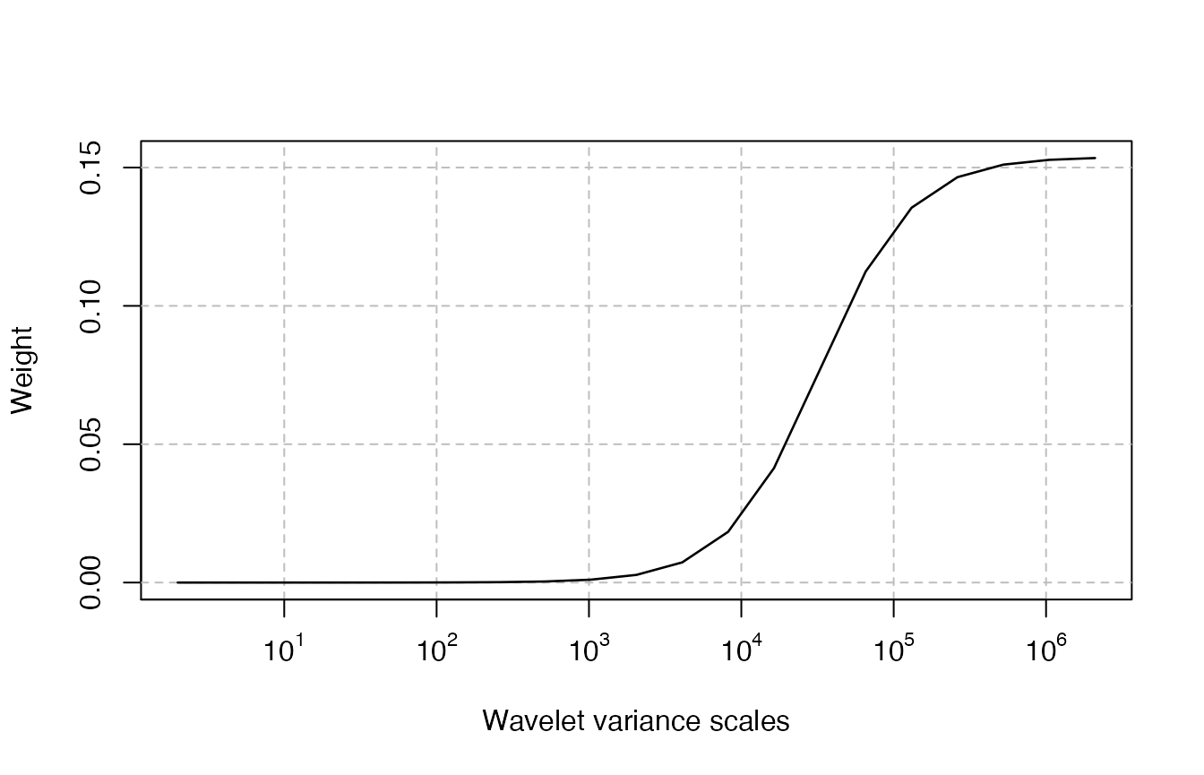
Once the weights on scales have been specified, one can obtain the coefficients to be used in the linear combination of single gyroscope signals as follows:
c_hat = find_optimal_coefs(Xt, weights)
c_hat
## [1] 0.043489268 0.016530619 0.029687293 0.103975706 0.069757839 0.219428143
## [7] 0.005264892 0.035700749 0.173090431 0.016060061 0.112651638 0.174363362The obtained virtual gyroscope can be compared with what would be obtained with equal coefficients using the “plot_virtual_gyro” function:
plot_virtual_gyro(Xt, c_hat, names = "SVO")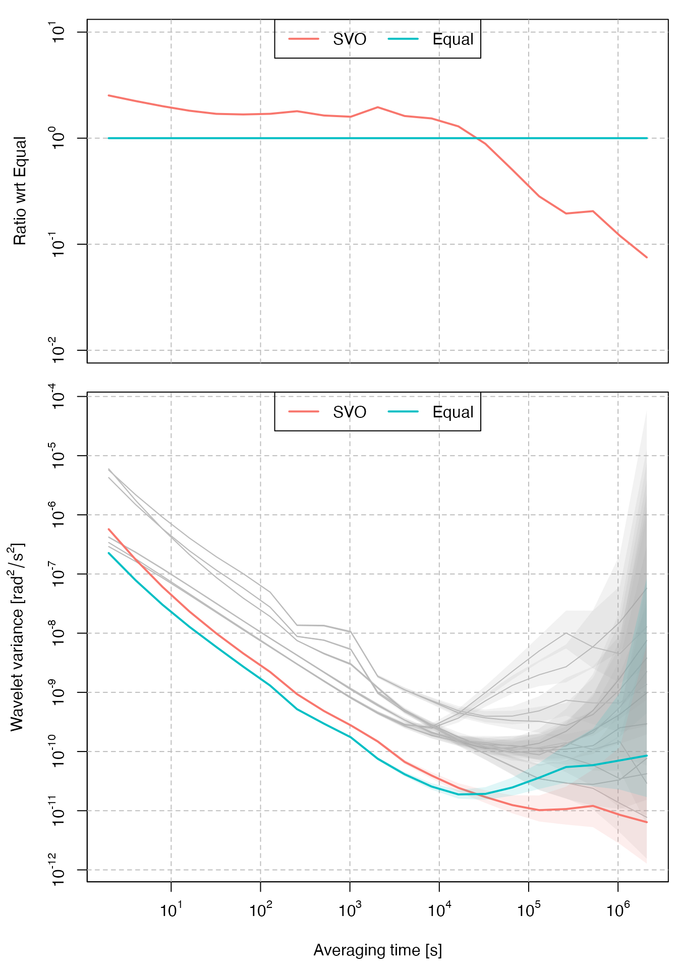
Simulation Studies
In this section we will provide the instructions on how to reproduce the Monte-Carlo simulations presented in Zhang et al. (2022).
White Noise + Random Walk
In this section we simulate data for six gyroscopes whose noise error model is composed by a white noise and a random walk (with correlated innovations), as in Equation (11) in Zhang et al. (2022).
# definition of the noise parameters

sigma_wn = c(2.805556e-07, 1.977778e-07, 1.361111e-07, 1.063889e-07, 1.069444e-07, 2.538889e-07)

sigma_rw = matrix(c(
  2.550583e-14, -8.573388e-16,  1.028807e-14, -1.628944e-14, -2.400549e-14, -5.572702e-15,
 -8.573388e-16,  4.715364e-14,  1.993313e-14,  1.071674e-15,  3.215021e-15,  2.079047e-14,
  1.028807e-14,  1.993313e-14,  3.489369e-13, -1.281722e-13,  5.572702e-15, -3.022119e-14,
 -1.628944e-14,  1.071674e-15, -1.281722e-13,  2.091907e-13,  4.093793e-14,  5.444102e-14,
 -2.400549e-14,  3.215021e-15,  5.572702e-15,  4.093793e-14,  5.551269e-14,  2.443416e-14,
 -5.572702e-15,  2.079047e-14, -3.022119e-14,  5.444102e-14,  2.443416e-14,  2.501286e-13
), nrow = 6, byrow = T)

N = 2^20

set.seed(1)
Xt = simulate_wn(N, sigma_wn) + simulate_corr_rw(N, sigma_rw)
We define weights in order to minimize the largest scales of the wavelet variance and we compute the coefficients with the approach of SVO:
n_scales = log2( N ) - 1
tau = 1:n_scales

weights = exp(tau-13)/(1 + exp(tau-13))
weights = weights/sum(weights)

c_svo = find_optimal_coefs(Xt, weights)
c_svo
## [1] 0.64883444 0.09086595 -0.08442475 -0.03256908 0.42664989 -0.04935644As a comparison, we also compute the optimal coefficients according to the method presented in Vaccaro and Zaki (2017), which can be calculated as follows:
# Estimate the Q matrix (the covariance of the Random Walk innovations)
Q_hat = algorithm_2(Xt)$Q

# Compute the coefficients
c_vaccarozaki = find_optimal_coefs_vaccaro(Q_hat)
c_vaccarozaki
## [1] 0.660701354 0.023822495 -0.035308980 -0.023871239 0.375950202
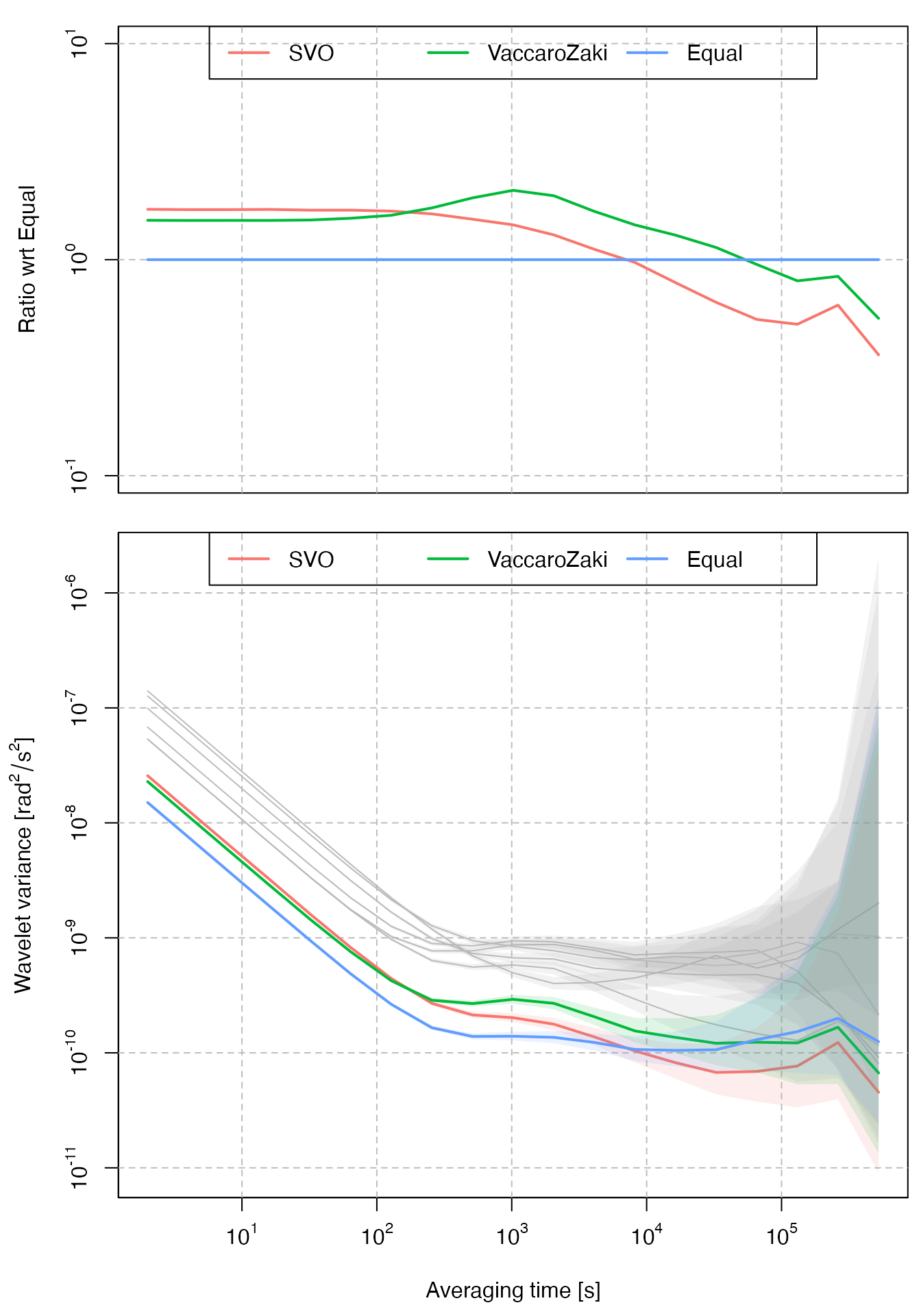
## [6] -0.001293832The results can be seen in the following plot. In this case, since the assumed model for the simulated gyroscopes satisfies the parametric assumptions in Vaccaro and Zaki (2017), the results of both approaches are mostly similar.
plot_virtual_gyro(Xt, c_svo, c_vaccarozaki, names = c("SVO", "VaccaroZaki"))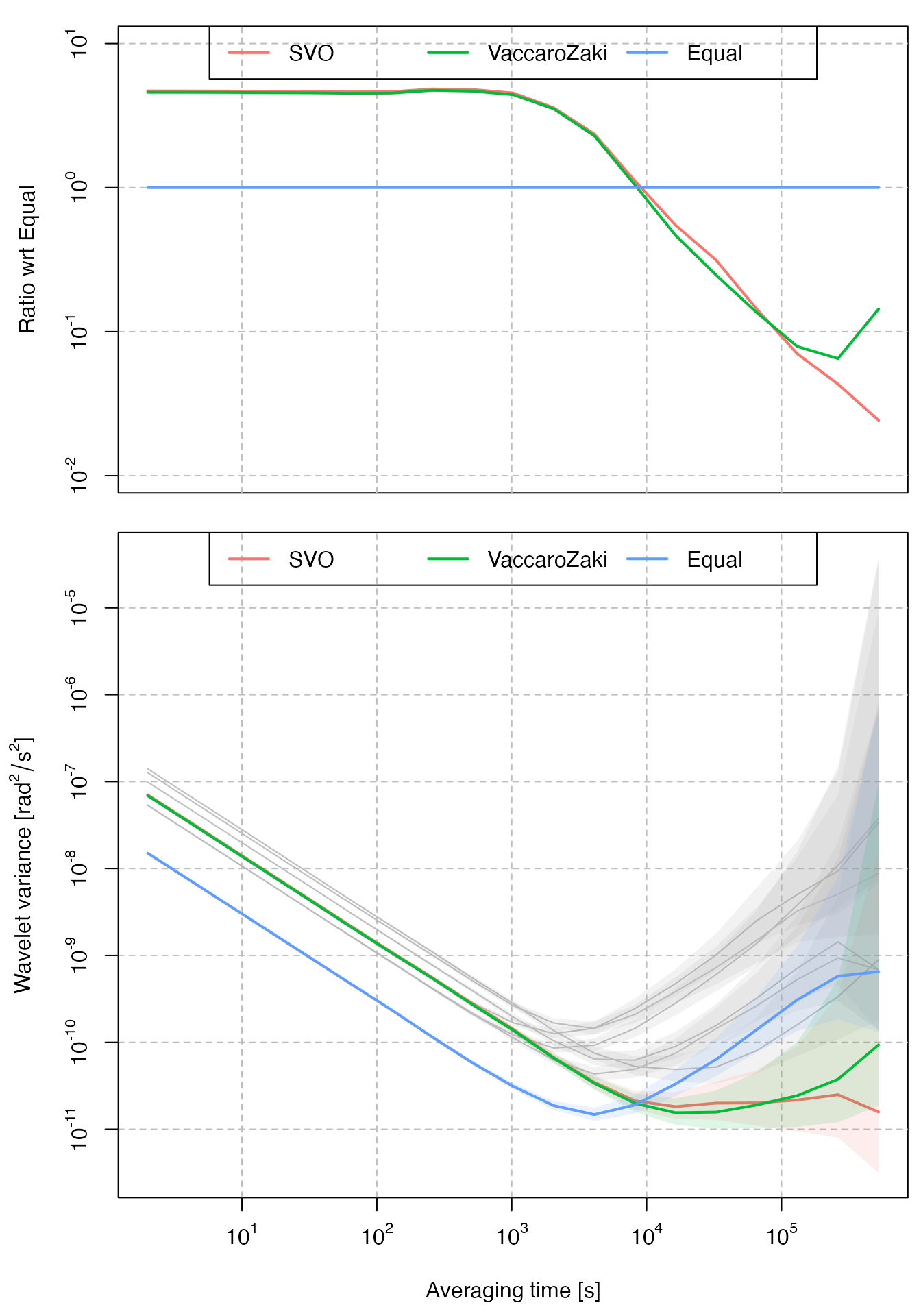
White Noise + 3 correlated AR(1)
In this example we simulate data for six gyroscopes whose noise error model is composed by a white noise and three first-order auto-regressive processes (with correlated innovations), as in Equation (14) in Zhang et al. (2022).
phi_ar1_1 = rep(0.9998705, 6)

sigma_ar1_1 = matrix(c(
  6.713833e-13,  1.515552e-13,  1.245013e-13, -7.117931e-15,  4.284888e-14,  9.577566e-14,
  1.515552e-13,  5.607230e-13,  2.264650e-13, -7.737235e-14,  2.810539e-14,  1.440987e-13,
  1.245013e-13,  2.264650e-13,  7.499051e-13, -1.626870e-14, -5.293172e-14, -9.995748e-14,
 -7.117931e-15, -7.737235e-14, -1.626870e-14,  1.207920e-13, -1.873054e-14,  6.817015e-14,
  4.284888e-14,  2.810539e-14, -5.293172e-14, -1.873054e-14,  7.499327e-13,  2.414762e-13,
  9.577566e-14,  1.440987e-13, -9.995748e-14,  6.817015e-14,  2.414762e-13,  6.461646e-13
), nrow = 6, byrow = T)

phi_ar1_2 = rep(0.9975214, 6)

sigma_ar1_2 = matrix(c(
  4.008129e-12, -1.806110e-13, -4.477015e-13, -1.048567e-12,  2.546714e-12, -2.349504e-12,
 -1.806110e-13,  1.177847e-11, -1.290506e-13, -3.741980e-12, -5.110108e-13,  2.849421e-12,
 -4.477015e-13, -1.290506e-13,  1.965775e-11,  2.026288e-12, -1.750890e-12,  1.446290e-12,
 -1.048567e-12, -3.741980e-12,  2.026288e-12,  1.309887e-11,  2.317561e-13,  4.127606e-12,
  2.546714e-12, -5.110108e-13, -1.750890e-12,  2.317561e-13,  1.928375e-11,  5.714532e-12,
 -2.349504e-12,  2.849421e-12,  1.446290e-12,  4.127606e-12,  5.714532e-12,  1.434466e-11
), nrow = 6, byrow = T)

phi_ar1_3 = rep(0.9999933, 6)

sigma_ar1_3 = matrix(c(
  5.062006e-14, -6.432804e-15,  3.260125e-15,  6.977995e-15,  1.727949e-14,  7.385838e-15,
 -6.432804e-15,  1.612038e-14, -3.184490e-15, -3.836343e-15, -7.682144e-15, -1.000440e-15,
  3.260125e-15, -3.184490e-15,  2.102923e-14,  9.145839e-16,  3.985049e-15, -1.377599e-15,
  6.977995e-15, -3.836343e-15,  9.145839e-16,  7.881771e-15, -1.291789e-15,  5.191186e-15,
  1.727949e-14, -7.682144e-15,  3.985049e-15, -1.291789e-15,  5.442670e-14,  3.786316e-15,
  7.385838e-15, -1.000440e-15, -1.377599e-15,  5.191186e-15,  3.786316e-15,  4.990004e-14
), nrow = 6, byrow = T)

set.seed(1)
Xt = simulate_wn(N, sigma_wn) +
  simulate_corr_ar1(N, phi_ar1_1, sigma_ar1_1) +
  simulate_corr_ar1(N, phi_ar1_2, sigma_ar1_2) +
  simulate_corr_ar1(N, phi_ar1_3, sigma_ar1_3)
We again estimate the coefficients for the virtual gyroscopes with the SVO approach and the method proposed in Vaccaro and Zaki (2017) and compare the results. In this case, SVO, which does not rely on any parametric assumption on the underlying stochastic processes, achieves better results.
c_svo = find_optimal_coefs(Xt, weights)
c_svo
## [1] -0.01993349 0.28989108 0.07229865 0.54648993 0.13307622 -0.02182240
# Estimate the Q matrix (the covariance of the Random Walk innovations)
Q_hat = algorithm_2(Xt)$Q

# Compute the coefficients
c_vaccarozaki = find_optimal_coefs_vaccaro(Q_hat)
c_vaccarozaki
## [1] 0.01690066 0.07819669 0.28049420 0.50242681 -0.03989131 0.16187295
plot_virtual_gyro(Xt, c_svo, c_vaccarozaki, names = c("SVO", "VaccaroZaki"))